Rhino Grasshopper Generative Design: A Practical Guide

Designing a bridge for hilly terrain or optimizing a complex viaduct structure isn't something you solve with a single sketch. These problems have hundreds of variables, load paths, material constraints, site geometry, clearance requirements, and the best solution often isn't the most obvious one. Rhino Grasshopper generative design gives engineers and architects a way to explore thousands of design alternatives simultaneously, letting algorithms handle the iteration while humans focus on judgment and decision-making.

If you work in Indian infrastructure, roads, bridges, tunnels, buildings, you've likely seen generative design outputs showing up in DPRs and technical submissions. NHAI bridge packages, metro station roofing, and irrigation headworks are all seeing computational design approaches move from niche experiment to practical workflow. Understanding how these tools work isn't just academic; it directly affects how projects get designed, valued, and built.

This guide walks you through the practical side of setting up and running generative design workflows in Rhino and Grasshopper. You'll learn how the parametric environment works, how to define design goals and constraints, how to connect solvers like Galapagos and Octopus, and how to evaluate results that actually make sense for real projects. No prior Grasshopper experience is assumed, but a basic familiarity with Rhino's modeling environment will help. At Arched, we work with infrastructure contractors every day, helping them find and qualify for the right tenders through AI-driven eligibility intelligence, and we built this resource because the tools shaping how projects are designed deserve the same clarity we bring to how they're procured.

What generative design means in Rhino and Grasshopper

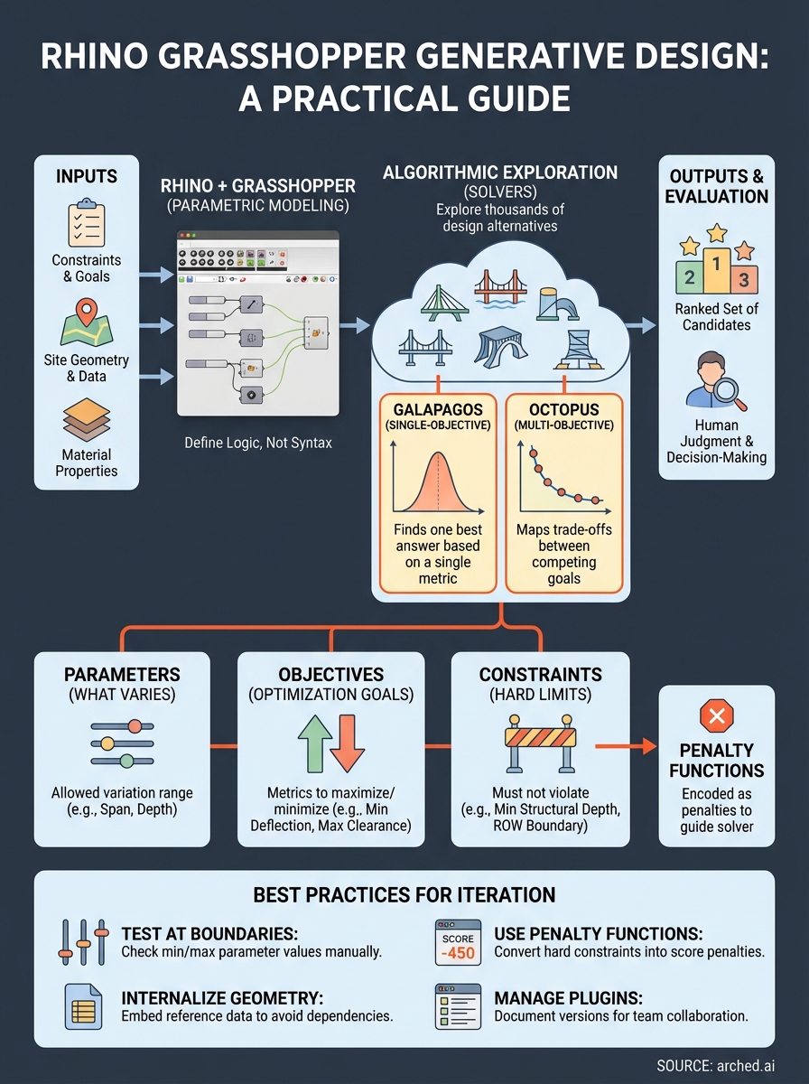
Generative design is a process where design constraints and performance goals drive a computational search across hundreds or thousands of possible forms, rather than a human manually testing each one. In Rhino and Grasshopper, this means you define a parametric model, specify what "better" looks like through objective functions, and let an algorithm explore the design space. The output isn't a single answer; it's a ranked set of candidates that you evaluate with engineering judgment before making a decision.

How Grasshopper works as a visual programming environment

Grasshopper runs inside Rhino as a node-based visual programming editor. Instead of writing code line by line, you connect components with wires to build a data flow that generates geometry. Each component takes inputs, performs an operation, and passes outputs forward. A simple example: a "Number Slider" component feeds a value into a "Move" component, which shifts a surface by that distance. Adjusting the slider updates the geometry in real time inside Rhino's viewport.

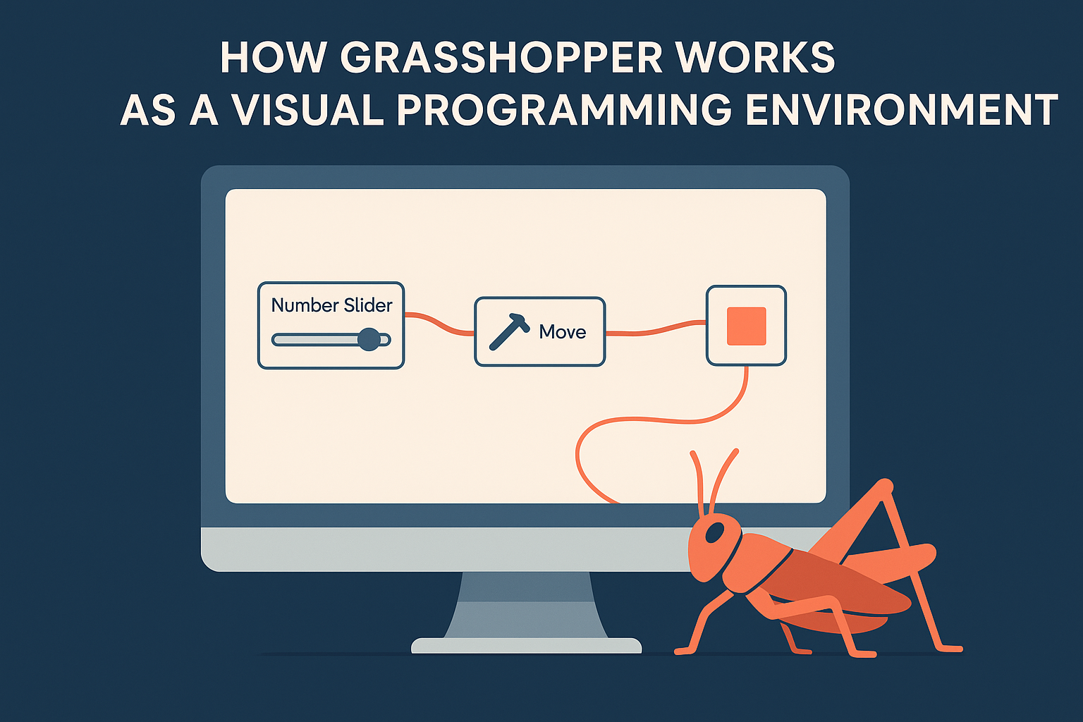
This visual structure is what makes rhino grasshopper generative design accessible to engineers and architects without a software development background. You're building logic, not writing syntax. When you connect a solver like Galapagos, Grasshopper's built-in single-objective optimizer, the slider values become genes that the algorithm mutates and recombines to find combinations that minimize or maximize your chosen metric.

Parameters, objectives, and constraints

These three inputs together define every generative design workflow you'll run in Grasshopper. Understanding the difference between them before you build anything saves significant time debugging later.

| Input type | What it defines | Bridge deck example | |---|---|---| | Parameters | What the algorithm is allowed to vary | Girder depth, span length, bearing spacing | | Objectives | What you are optimizing for | Minimize deflection, maximize clearance | | Constraints | Hard limits the design cannot violate | Minimum structural depth, ROW boundary |

Parameters get a defined range and a step size. If girder depth can range from 1.2 m to 2.4 m in 100 mm increments, that single parameter gives the solver thirteen possible values to work with. Multiply that across six or eight parameters and you have a search space far too large to navigate manually, which is exactly the point.

The clearest way to think about it: parameters define what can change, objectives define what you're optimizing for, and constraints define what can never be violated regardless of the optimization score.

Your objective function is how the solver scores each candidate design. The solver generates a candidate, evaluates it against the function, uses the score to guide the next generation of candidates, and repeats. The more precisely you encode your performance goals into that function, the more useful the output becomes.

What generative design is not

Generative design in Grasshopper is not a button you press to receive a finished design. The algorithm doesn't understand structural behavior, buildability, or site context unless you encode those things explicitly into your model. If your objective function only measures surface area, the solver optimizes for surface area, regardless of whether the result is structurally sound or constructible.

It is also not the same as simply having a parametric model. A parametric model lets you change values manually and watch the geometry update; generative design automates the systematic search through those values. The distinction matters in practice. A model with fifteen sliders gives you more possible combinations than you can explore manually in a week. Connecting it to a solver turns that parametric flexibility into a structured search with a clear evaluation criterion at every step. One is a drafting tool you control directly; the other is a search process you set up and supervise.

Set up Rhino and Grasshopper for iteration

Before you run a single solver, your Rhino and Grasshopper workspace needs to support fast iteration from the start. A disorganized canvas slows every workflow you build on top of it. The setup steps below apply whether you're optimizing a bridge girder cross-section or exploring structural bay spacing for a large-span roof.

Install and configure your environment

Grasshopper ships bundled with Rhino 6 and later, so no separate installation is required if you're on a current license. Open Grasshopper from the Rhino command line by typing Grasshopper and pressing Enter. For rhino grasshopper generative design workflows that go beyond manual slider adjustment, you need two solver plugins: Galapagos handles single-objective optimization and is already bundled with Grasshopper; Octopus handles multi-objective problems and requires a separate install through the Rhino package manager.

Follow this sequence before opening your first definition:

1. Set your Rhino unit system to match your project (meters for infrastructure work, millimeters for detailed components). Grasshopper inherits this unit context directly.
2. Enable automatic saving in Grasshopper preferences. Solver runs can crash unexpectedly, and you want your last working state recoverable.
3. Install the Human UI plugin if you plan to share definitions with team members who are not building in Grasshopper themselves. It lets you create clean input panels without exposing the full canvas.
4. Set solver geometry preview to off by default in the Grasshopper display menu. Rendering geometry for every candidate during a run adds significant processing time with no benefit during optimization.

Turning off geometry preview during solver runs alone can cut iteration time by 30 to 60 percent on complex definitions, depending on mesh density and component count.

Structure your canvas for iteration

Canvas organization directly affects how quickly you can debug a definition and how reliably it runs during optimization. Group your components into three horizontal zones: inputs on the left, geometry logic in the center, and outputs and objective functions on the right. Use Grasshopper's native Group and Scribble tools to label each zone clearly. This layout makes it immediately obvious where a solver reads parameter values and where it reads fitness scores.

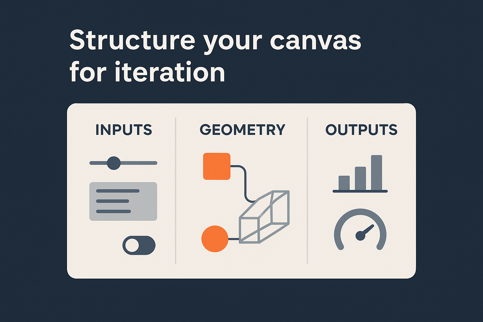
Your inputs zone should contain only number sliders, panels, and toggle switches that the solver or a team member needs to interact with directly. Move all intermediate geometry components out of this zone. When Galapagos or Octopus scans the canvas for genes to vary, a clean input zone prevents accidental connections to the wrong components and makes the gene assignment step faster and less error-prone.

Build a parametric model you can trust

A parametric model that fails mid-optimization is more damaging than no parametric model at all. When Galapagos or Octopus runs thousands of candidates, it cannot pause to ask you whether a specific geometry combination is physically valid. If your definition produces null geometry, inverted surfaces, or division-by-zero errors at certain parameter values, the solver either crashes or silently passes over valid regions of your design space. Building a model that handles its full parameter range without errors is the prerequisite for any generative design workflow in Rhino Grasshopper.

Keep your geometry logic flat and testable

Nested data trees are the most common source of silent errors in Grasshopper definitions. When you feed a list of curves into a component that expects a single curve, Grasshopper often produces output rather than throwing an error, but the output is not what you intended. Keep your geometry operations as shallow as possible: work with individual items before branching into lists, and use the Path Mapper component only when you have a clear reason for restructuring your data tree.

Before connecting any solver, run manual checks across your parameter range by dragging sliders to their minimum, midpoint, and maximum values and inspecting the geometry in Rhino's viewport. For a bridge girder definition, this means checking that the deck surface remains valid when girder depth is at its smallest, span is at its longest, and bearing spacing is at its widest. If any combination produces a warning or null output, fix it before the solver sees it. The table below shows the three-point check approach for a simple bridge parameter set:

| Parameter | Min value | Mid value | Max value | |---|---|---|---| | Girder depth | 1.2 m | 1.8 m | 2.4 m | | Span length | 20 m | 35 m | 50 m | | Bearing spacing | 2.0 m | 3.5 m | 5.0 m |

Test every corner of your parameter space manually before connecting a solver. Errors at boundary values will derail optimization runs that could otherwise take hours to complete.

Use internalized geometry to reduce external dependencies

Rhino Grasshopper generative design definitions break when the Rhino file they reference gets moved, renamed, or updated. Avoid this by internalizing reference geometry directly inside the Grasshopper definition: right-click any geometry component and select "Internalize Data." This embeds the geometry into the definition itself, so it runs correctly on any machine regardless of which Rhino file is open. For site boundaries, alignment curves, or fixed structural reference points, internalization eliminates an entire category of errors that appear only when someone else opens your file or when you run the definition on a different workstation.

Add constraints and performance metrics

Constraints and performance metrics are what separate a useful rhino grasshopper generative design workflow from one that generates geometrically valid but practically useless results. Without them, your solver explores the full parameter space with no knowledge of what "better" actually means for your project. Defining these inputs precisely before you run optimization is not optional; it determines whether the output candidates are worth evaluating at all.

Encode hard constraints as penalty functions

Grasshopper has no native mechanism to exclude parameter combinations from a solver run before they are evaluated. You handle this by encoding hard constraints as penalty values that spike the objective function score when a design violates a limit. The solver then learns to avoid those regions because they score poorly, not because they were blocked from the start.

A straightforward penalty pattern in Grasshopper uses the native Mass Addition and Multiplication components to add a large negative (or positive, depending on your optimization direction) value to the fitness score when a parameter combination crosses a threshold. Here's the logic for a structural clearance constraint:

IF deck_soffit_elevation < minimum_clearance
  THEN fitness = fitness + (-1000000)
ELSE
  THEN fitness = fitness + 0

Wire this pattern for every hard constraint in your definition and connect the summed penalty output to the same fitness input as your performance score. The combined value becomes what the solver minimizes or maximizes.

Keep penalty magnitudes at least two orders larger than your normal fitness range so a constraint violation always dominates the score, regardless of how well the design performs on other metrics.

Define your performance metrics

Your performance metrics are the objective functions the solver actively optimizes toward. These are distinct from constraints: constraints rule out invalid designs, while metrics rank valid ones. For infrastructure work, common metrics include structural material volume (as a proxy for cost), mid-span deflection under live load, or floor area efficiency for building projects.

Grasshopper evaluates metrics using analysis components. Karamba3D handles structural analysis for deflection, stress, and utilization directly within a Grasshopper definition without exporting to a separate FE package. For thermal or daylighting metrics, Ladybug Tools integrates environmental analysis into the same canvas. Both return numeric outputs you can wire directly into a fitness function.

| Metric type | Grasshopper source | Optimization direction | |---|---|---| | Material volume | Mass Properties component | Minimize | | Mid-span deflection | Karamba3D Analyze component | Minimize | | Usable floor area | Area component | Maximize | | Solar exposure | Ladybug Radiation Analysis | Maximize or minimize |

Connect your chosen metric output to the fitness input of your solver component. If you are running multi-objective optimization in Octopus, wire each metric to a separate fitness input rather than combining them into a single score. Octopus generates a Pareto front across all objectives simultaneously, giving you a set of candidates where improving one metric requires a trade-off against another.

Generate options with search and optimization

With your parametric model tested and your constraints and metrics wired correctly, you are ready to run the solver. Galapagos and Octopus approach the search differently, and choosing the right one for your problem determines whether the output is useful or misleading. Galapagos searches for a single best answer; Octopus maps the full trade-off surface between competing objectives. Both tools read your parameter sliders as genes and your fitness function output as the score they are trying to improve.

Run Galapagos for single-objective problems

Galapagos is the right choice when you have one clear metric to optimize and your constraints are already encoded as penalty functions. Open the Galapagos component from the Grasshopper toolbar under the Params tab, connect your slider components to the Genome input, and connect your fitness output to the Fitness input. Then double-click the component to open the solver window.

Set these parameters before your first run:

• Population size: Start at 50 for fast exploration. Increase to 100 or 150 for complex definitions with more than eight genes.
• Max generations: Set 100 as an initial limit. You can extend the run if the fitness curve is still improving when it stops.
• Maintain population: Keep this enabled. It preserves the best candidates across restarts, so you do not lose progress if you pause and resume.

Watch the fitness curve during the run. If it plateaus before generation 40, your penalty functions may be too aggressive, blocking the solver from reaching valid regions of the parameter space.

Once the run completes, Galapagos holds the best-found parameter combination in your sliders. Record those values in a Grasshopper panel before running again, because the next run overwrites them.

Run Octopus for multi-objective problems

Octopus generates a Pareto front instead of a single best answer, which makes it the correct tool for any problem where improving one metric forces a trade-off against another. A bridge deck optimization balancing material volume against mid-span deflection is a typical case. Wire each fitness output to a separate Fitness input on the Octopus component, then connect your sliders to the Genome input exactly as you would for Galapagos.

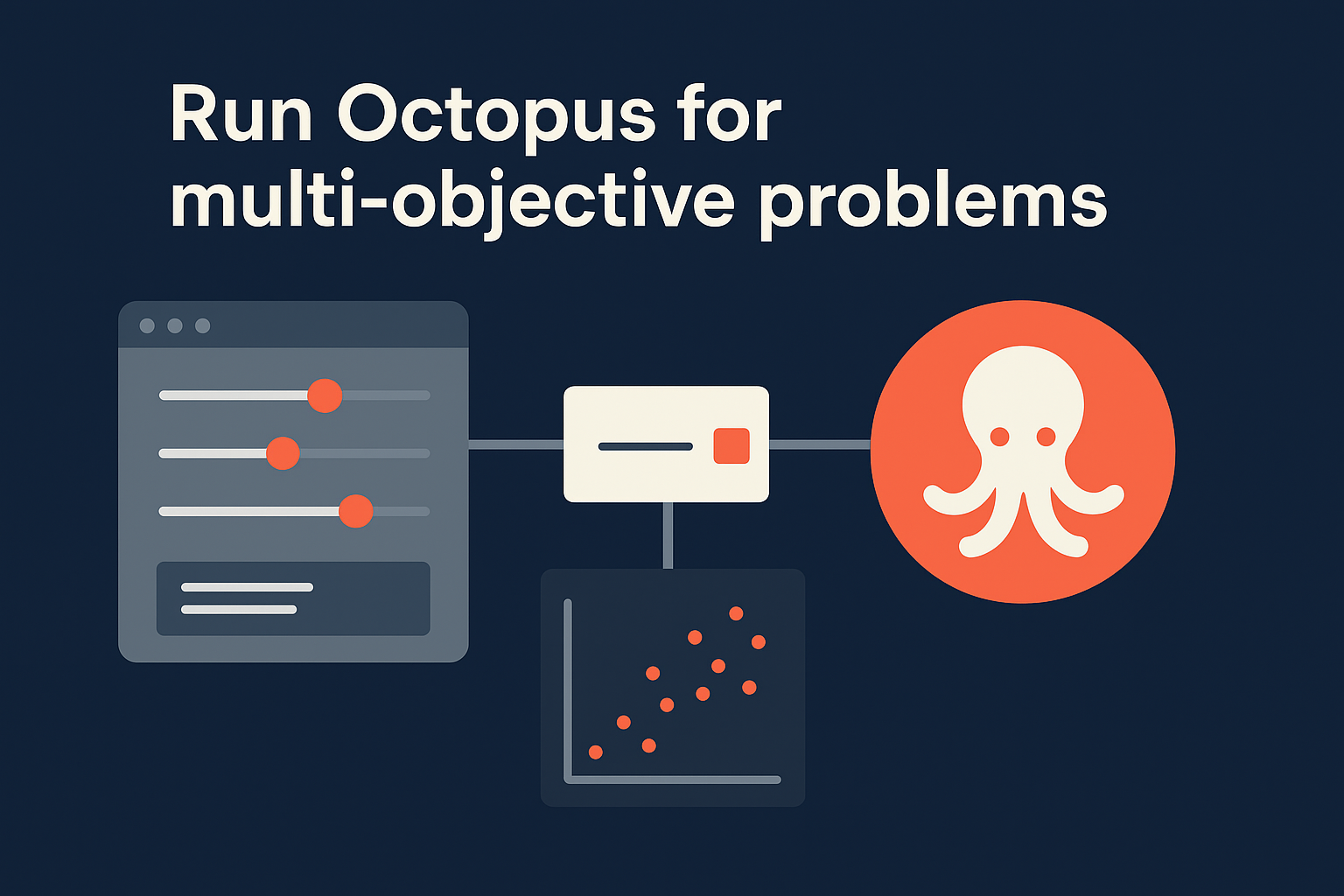
After the run, Octopus displays the Pareto front as a point cloud in its results window. Each point is a fully valid design candidate. Your task at this stage is to apply engineering judgment to select the candidates worth extracting: export the slider values for your top three to five candidates into separate named panels, then bake the corresponding geometry into Rhino for downstream evaluation. The rhino grasshopper generative design workflow gives you the candidates; you make the final call on which ones move forward.

Troubleshoot and scale your workflow

Most solver failures in rhino grasshopper generative design workflows trace back to two sources: geometry that breaks at boundary parameter values, and fitness functions that return null instead of a number. When Galapagos or Octopus encounters a null fitness output, it does not skip the candidate; it treats the result as the worst possible score and moves on. The solver keeps running, but the regions that produced nulls get flagged as low-fitness, and valid design space near those boundaries may go entirely unexplored. Catching these errors before a long run saves hours you cannot recover.

Fix the most common solver failures

The fastest way to locate null-producing parameter combinations is to add a Grasshopper error detection step directly upstream of your fitness output. Use the native "Is Null" component on every geometry output that feeds your analysis chain, then wire those Boolean flags into a Mass Addition component. If the sum is greater than zero, pipe a large penalty value into your fitness score. This converts a silent null into a visible, traceable penalty event you can isolate by reviewing your parameter history after the run.

Review your parameter history log after every solver run, not just when something looks wrong. Patterns in the failed candidates often reveal which parameter boundaries are producing the errors.

Common error sources and their fixes:

| Error | Cause | Fix | |---|---|---| | Null fitness output | Analysis component receives invalid geometry | Add Is Null check before analysis chain | | Solver stalls at generation 1 | All candidates violate constraints | Reduce penalty magnitude or widen parameter range | | Duplicate candidates on Pareto front | Parameter step size too coarse | Reduce slider step size by half | | Definition crashes mid-run | Memory overload from dense mesh preview | Disable mesh preview before starting solver |

Scale across a project team

When your definition works reliably on a single machine, your next challenge is sharing it without breaking it. Grasshopper definitions reference external plugins by name, and any team member who opens your file without the same plugin versions installed sees missing components and an inoperable canvas. Before distributing a definition, document every non-native plugin your canvas uses, its version number, and its installation source inside a Scribble note placed at the top of the canvas.

For teams running the same definition across multiple active tenders, version control matters more than it appears. Store your Grasshopper definition files in a shared folder with a clear naming convention: ProjectCode_DefinitionPurpose_Version.gh. Treat each tested, approved version as a release, and never overwrite a working file with an experimental change. This protects your team from losing a stable solver configuration because someone updated a component that was already performing correctly.

Next steps

You now have a complete foundation for running rhino grasshopper generative design workflows from setup through solver output. The practical path forward is to start with one real project parameter, a single span length or girder depth range, and build your first Galapagos run around it. A small, working definition teaches you more than reading documentation for hours, because you encounter the actual error messages and data tree issues that appear on your specific geometry.

Once your first run produces usable candidates, extend the same approach to multi-objective problems using Octopus. Add Karamba3D for structural metrics, test your penalty functions against boundary values, and document every plugin version before sharing with your team. Each completed workflow becomes a reusable template for the next project type.

If you work in Indian infrastructure procurement and want to understand how computational design intersects with tender eligibility, explore Arched's infrastructure intelligence platform to see how project credentials map against NHAI and other authority requirements.